Supercharging Hyperparameter Tuning with Dask
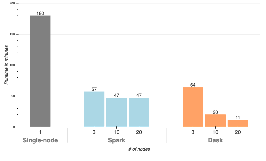
TL;DR: Dask improves scikit-learn parameter search speed by over 16x, and Spark by over 4x.

Hyperparameter tuning is a crucial, and often painful, part of building machine learning models. Squeezing out each bit of performance from your model may mean the difference of millions of dollars in ad revenue or life-and-death for patients in healthcare models. Even if your model takes one minute to train, you can end up waiting hours for a grid search to complete (think a 10×10 grid, cross-validation, etc.). Each time you wait for a search to finish breaks an iteration cycle and increases the time it takes to produce value with your model. Shortly put:
- Faster runtime means more iterations to improve accuracy before your deadline
- Faster runtime means quicker delivery so you can tackle another project
- Both bullet points mean driving value to the bottom line of your organization
In this post we will see show how you can improve the speed of your hyperparameter search by over 16x by replacing a few lines of your scikit-learn pipeline with Dask code on Saturn Cloud. This turns a traditionally overnight parameter search to a matter of waiting a few seconds. We also try a comparable grid search with Apache Spark which requires significantly more code change while still being much slower than Dask.
First, what is Dask?
Dask is a
flexible and robust parallel computing framework built-in, and for,
Python. It works with common data
structures such
as Arrays and DataFrames, but can also be used to parallelize complex
operations that do not fit nicely into those. In fact, the parallel
Arrays and DataFrames are actually collections of
familiar numpy and pandas objects, and have
matching APIs. This way, data scientists do not need to learn entirely
new frameworks to be able to execute their code on big
data.
Experiment setup
We will use the publicly available NYC Taxi dataset and train a linear regression model that can predict the fare amount of a taxi ride using attributes related to rider pickup.
We’ll first walk through the data loading and grid search using
single-node Python packages (pandas and scikit-learn), and then
highlight what changes are required to parallelize the grid search with
Dask or Spark. All three workloads perform the same grid search with the
same data, and we will refer to them throughout the article as
Single-node (for single-node Python), Dask (for Dask
cluster), and Spark (For Spark cluster).
Hardware
For all tasks, we use r5.2xlarge instances from AWS (8 cores, 64GB RAM). For Python, we only use one node, and for Spark and Dask we run the workload on clusters with different numbers of worker nodes to track the runtime (3, 10, and 20).
Spark clusters are managed using Amazon EMR, while Dask clusters are managed using Saturn Cloud.
Just show me the results!
If you want to skip the code and see the performance improvements, jump down to the Results section.
Single-node workflow
First, load the data! We randomly sample the data for benchmark purposes.
import pandas as pd
import numpy as np

taxi = pd.read_csv(
    's3://nyc-tlc/trip data/yellow_tripdata_2019-01.csv',
    parse_dates=['tpep_pickup_datetime', 'tpep_dropoff_datetime'],
).sample(frac=0.1, replace=False)
Then, create some features:
taxi['pickup_weekday'] = taxi.tpep_pickup_datetime.dt.weekday
taxi['pickup_weekofyear'] = taxi.tpep_pickup_datetime.dt.weekofyear
taxi['pickup_hour'] = taxi.tpep_pickup_datetime.dt.hour
taxi['pickup_minute'] = taxi.tpep_pickup_datetime.dt.minute
taxi['pickup_year_seconds'] = (taxi.tpep_pickup_datetime - datetime.datetime(2019, 1, 1, 0, 0, 0)).dt.seconds
taxi['pickup_week_hour'] = (taxi.pickup_weekday * 24) + taxi.pickup_hour
taxi['passenger_count'] = taxi.passenger_count.astype(float).fillna(-1)
taxi = taxi.fillna(value=)

# keep track of column names for pipeline steps
numeric_feat = ['pickup_weekday',  'pickup_weekofyear', 'pickup_hour', 'pickup_minute', 'pickup_year_seconds', 'pickup_week_hour',  'passenger_count']
categorical_feat = ['VendorID', 'RatecodeID', 'store_and_fwd_flag', 'PULocationID', 'DOLocationID']
features = numeric_feat + categorical_feat
y_col = 'total_amount'
We are using a scikit-learn Elastic
Net model,
which can perform L1, L2 and ElasticNet regularization based on
the l1_ratio parameter. We’ll also try a few values
of alpha, creating a grid with 404 items and 3-fold
cross-validation, resulting in 1,212 model fits for the
search.
As we’re training a linear model, we need to one-hot encode the
categorical features and scale the numeric features. Note
the n_jobs=-1 parameter when defining the GridSearchCV instructs
scikit-learn to parallelize the model training across all the cores in
the machine (this doesn’t use Dask yet, as the single-node
parallelization comes out-of-the-box with
scikit-learn).
from sklearn.pipeline import Pipeline
from sklearn.linear_model import ElasticNet
from sklearn.compose import ColumnTransformer
from sklearn.preprocessing import StandardScaler, OneHotEncoder
from sklearn.model_selection import GridSearchCV

pipeline = Pipeline(steps=[
    ('preprocess', ColumnTransformer(transformers=[
        ('num', StandardScaler(), numeric_feat),
        ('cat', OneHotEncoder(handle_unknown='ignore', sparse=False), categorical_feat),
    ])),
    ('clf', ElasticNet(normalize=False, max_iter=100)),
])

# this is our grid
params = {
    'clf__l1_ratio': np.arange(0, 1.01, 0.01),
    'clf__alpha': [0, 0.5, 1, 2],
}

grid_search = GridSearchCV(pipeline, params, cv=3, n_jobs=-1, scoring='neg_mean_squared_error')
Finally, we can run the grid search and retrieve the best score:
grid_search.fit(taxi[features], taxi[y_col])
print(grid_search.best_score_)
If you were to run this on a similarly-sized machine as we did it would take approximately 3 hours.
Drop-In Dask
Dask will run great on a single-node and can scale to clusters with
thousands of nodes. To start using Dask, we need to initialize a client, and in
this case we will set up our
cluster using
Saturn Cloud’s SaturnCluster.
from dask.distributed import Client
from dask_saturn import SaturnCluster

cluster = SaturnCluster(n_workers=20)
client = Client(cluster)
The only change we need to make when reading the data is to use
the dask.dataframe package instead of pandas. All the feature
engineering code remains exactly the same because Dask Dataframes implement the pandas
API.
import dask.dataframe as dd

taxi = dd.read_csv(
    's3://nyc-tlc/trip data/yellow_tripdata_2019-01.csv',
    parse_dates=['tpep_pickup_datetime', 'tpep_dropoff_datetime'],
).sample(frac=0.1, replace=False)
Then to create our pipeline and grid search:
from dask_ml.compose import ColumnTransformer
from dask_ml.preprocessing import StandardScaler, DummyEncoder, Categorizer
from dask_ml.model_selection import GridSearchCV

# Dask has slightly different way of one-hot encoding
pipeline = Pipeline(steps=[
    ('categorize', Categorizer(columns=categorical_feat)),
    ('onehot', DummyEncoder(columns=categorical_feat)),
    ('scale', ColumnTransformer(transformers=[('num', StandardScaler(), numeric_feat)],
        remainder='passthrough')),
    ('clf', ElasticNet(normalize=False, max_iter=100)),
])

# params same as above
grid_search = GridSearchCV(pipeline, params, cv=3, scoring='neg_mean_squared_error')
Note that Dask has a couple different classes for preprocessing
and GridSearchCV, which are used to speed up pre-processing and avoid
unnecessary re-computation during the grid search. The pipeline and
estimator (ElasticNet) classes
are used directly from scikit-learn.
We can fit the grid search the same way as we did with the single-node scikit-learn:
grid_search.fit(taxi[features], taxi[y_col])
print(grid_search.best_score_)
Running this grid search using 20 nodes results in a runtime of 11 minutes! That a 16x improvement by just changing ~10 lines of code. Let me be dramatic and say that again.
16x improvement by changing 10 lines of code!
Spark
Apache Spark is a big data processing engine built in Scala with a Python interface that calls down to the Scala/JVM code. It’s a staple in the Hadoop processing ecosystem, built around the MapReduce paradigm, and has interfaces for DataFrames as well as machine learning.
To run our workload with Spark, we need to refactor our Python code to use Spark’s DataFrame as well as Spark ML pipelines, preprocessing, and model classes.
from pyspark.sql import SparkSession

spark = SparkSession.builder.getOrCreate()

taxi = spark.read.csv('s3://nyc-tlc/trip data/yellow_tripdata_2019-01.csv',
                      header=True,
                      inferSchema=True,
                      timestampFormat='yyyy-MM-dd HH:mm:ss',
                    ).sample(fraction=0.1, withReplacement=False)
The feature engineering looks slightly different than pandas:
import pyspark.sql.functions as F
import pyspark.sql.types as T

taxi = taxi.withColumn('pickup_weekday', F.dayofweek(taxi.tpep_pickup_datetime).cast(T.DoubleType()))
taxi = taxi.withColumn('pickup_weekofyear', F.weekofyear(taxi.tpep_pickup_datetime).cast(T.DoubleType()))
taxi = taxi.withColumn('pickup_hour', F.hour(taxi.tpep_pickup_datetime).cast(T.DoubleType()))
taxi = taxi.withColumn('pickup_minute', F.minute(taxi.tpep_pickup_datetime).cast(T.DoubleType()))
taxi = taxi.withColumn('pickup_year_seconds',
                                    (F.unix_timestamp(taxi.tpep_pickup_datetime) -
                                    F.unix_timestamp(F.lit(datetime.datetime(2019, 1, 1, 0, 0, 0)))).cast(T.DoubleType()))
taxi = taxi.withColumn('pickup_week_hour', ((taxi.pickup_weekday * 24) + taxi.pickup_hour).cast(T.DoubleType()))
taxi = taxi.withColumn('passenger_count', F.coalesce(taxi.passenger_count, F.lit(-1)).cast(T.DoubleType()))
taxi = taxi.fillna()
# Spark ML expects a "label" column for the dependent variable
taxi = taxi.withColumn('label', taxi.total_amount)
Then, we set up our pre-processing pipeline and grid search. Spark ML
expects all features in a single vector column, so we
use VectorAssembler to
collect all our processed columns.
from pyspark.ml.regression import LinearRegression
from pyspark.ml.tuning import CrossValidator, ParamGridBuilder
from pyspark.ml.evaluation import RegressionEvaluator
from pyspark.ml.feature import OneHotEncoder, StringIndexer, VectorAssembler, StandardScaler
from pyspark.ml.pipeline import Pipeline

indexers = [
    StringIndexer(
    inputCol=c,
    outputCol=f'_idx', handleInvalid='keep')
    for c in categorical_feat
]
encoders = [
    OneHotEncoder(
        inputCol=f'_idx',
        outputCol=f'_onehot',
    )
    for c in categorical_feat
]
num_assembler = VectorAssembler(
    inputCols=numeric_feat,
    outputCol='num_features',
)
scaler = StandardScaler(inputCol='num_features', outputCol='num_features_scaled')

assembler = VectorAssembler(
    inputCols=[f'_onehot' for c in categorical_feat] + ['num_features_scaled'],
    outputCol='features',
)

lr = LinearRegression(standardization=False, maxIter=100)
pipeline = Pipeline(
    stages=indexers + encoders + [num_assembler, scaler, assembler, lr])

# this is our grid
grid = (
    ParamGridBuilder()
    .addGrid(lr.elasticNetParam, np.arange(0, 1.01, 0.01))
    .addGrid(lr.regParam, [0, 0.5, 1, 2])
    .build()
)

crossval = CrossValidator(estimator=pipeline,
                            estimatorParamMaps=grid,
                            evaluator=RegressionEvaluator(),
                            numFolds=3)
Then, we run our grid search and get the best result:
fitted = crossval.fit(taxi)
print(np.min(results.avgMetrics))  # min because metric is RMSE
On a 20 node cluster, this takes approximately 47 minutes.
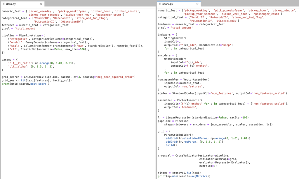
Here is a side by side look at the grid search code to give you a sense of how much easier Dask is in this example.
Code Volume: Dask (left) and Spark (right)

Results
We ran a hyperparameter search with 404 configurations and 3 folds of cross-validation, using an Elastic Net model to predict taxi trip duration from the NYC taxi dataset. We started off with a single-node Python implementation and transferred that to a cluster using Dask and Spark. We can see from the table below that the Dask search was drastically faster than the single-node and Spark cluster versions, while requiring minimal code changes.
| System | Runtime | LOC changed |
|---|---|---|
| Single-node | 3 hours | – |
| Dask | 11 minutes | 10 |
| Spark | 47 minutes | 100 |
We ran the Dask and Spark workloads on clusters of various sizes to see how a larger cluster improves parameter search time:

Why is Dask so fast?
Dask parallelizes the model fitting across the nodes and cores in the cluster, so you can expect an approximately linear speedup when adding more machines to the cluster. There is some overhead involved with parallelizing work, which is why we saw a 16x improvement by adding 19 machines.
Spark is much slower in this example because the Spark grid search implementation does not parallelize the grid, it only parallelizes the model fitting. This becomes a sequential grid search with portions in each fit parallelized across the cluster. There is a project, joblibspark, in active development, that seeks to parallelize scikit-learn pipelines on a Spark cluster. At the time of writing this post, we were unable to successfully run joblibspark.
All the code for this post is available here.
Do You Need Faster Hyperparameter Searches?
Yes! You can get going on a Dask cluster in seconds with Saturn Cloud. Saturn handles all the tooling infrastructure, security, and deployment headaches to get you up and running with Dask right away.
